01 ETL Pipelines
“Without a systematic way to start and keep data clean, bad data will happen.” — Donato Diorio
Source: Mindaugas Sadūnas
Table of Contents
- Overview
- Learning Outcomes
- Data
- Tools
- Data Pipelines
- 🐼
pipelines - Extract
- Transform
- Load
- Launch a Pipeline
- Summary
1. Overview
You are a data analyst working at Beautiful Analytics, and you have been given a project in which you will work using data generated from shared bikes systems in the cities of London (England, UK), Seoul (South Korea), and Washington (DC, USA). Your customer's are the governments of each city and what they want to solve is the same,
Challenge #1
To predict/forecast how many bikes they will to need to have available in the city at every hour of the dat for the next few years?
Each government captures similar data but, as you can imagine, they all use different words and measure similar variables in different ways. This means that our first job before we can answer the question above is to fix the data and put it in amore user-friendly way. While we are at it, we should also try and automate our pipeline so that the next time we need to read, transform, and load new versions of all the data sources for this project, we could do so with the click of a button rather than having to write everything again from scratch. So our first real problem is,
Challenge #0
Create a data pipeline that extracts, transforms and loads the necessary data for the task at hand.
2. Learning Outcomes
Before we get started, let's go over the learning outcomes for this section of the workshop.
By the end of this lesson you will be able to,
- Discuss what ETL and ELT Pipelines are.
- Understand how to read and combine data that comes from different sources.
- Create data pipelines using pandas and prefect.
- Understand how to visualize the pipelines you create to help you with their development.
3. Data

All three data files contain similar information about how many bicycles have been rented each hour, day, week and months for several years and for each city government we are working with.
You can get more information about the data of each city using the following links.
Here are the variables that appear in the three data files.
| London | Seoul | Washington |
|---|---|---|
| date | date | instant |
| count | count | date |
| temperature | hour | seasons |
| t2 | temperature | year |
| humidity | humidity | month |
| wind_speed | wind_speed | hour |
| weather_code | visibility | is_holiday |
| is_holiday | dew_point_temp | weekday |
| is_weekend | solar_radiation | workingday |
| seasons | rainfall | weathersit |
| snowfall | temperature | |
| seasons | count | |
| is_holiday | humidity | |
| functioning_day | wind_speed | |
| casual | ||
| registered |
Since all of these datasets where generated with different business logic and, most likely, by completely different systems, we can certainly expect more inconsistencies than just unmatching column names, numerical formats, and data collected. We will walk through a few cleaning steps after we discuss the tools we will be using today.
4. Tools
The tools that we will use in the workshop are the following.
- pandas - "is a fast, powerful, flexible and easy to use open source data analysis and manipulation tool, built on top of the Python programming language."
- Prefect - "is a new workflow management system, designed for a modern infrastructure and powered by the open source workflow engine, Prefect Core. Users organize tasks into
task's andflow's, and Prefect takes care of the rest." - sqlite3 - "SQLite is a library written in C that provides a lightweight disk-based database that does not require a separate server process and allows the database to be accessed using a non-standard variant of the SQL query language."
- pathlib - allows us to manipulate paths as if they were python objects.
Before we continue, let's load the modules we'll need and examine our datasets.
import pandas as pd
from prefect import flow, task
import sqlite3
from contextlib import closing
from pathlib import Path


pd.options.display.max_rows = None
pd.options.display.max_columns = None
path = Path().cwd().parent.joinpath("data", "01_part")
path
We will need paths to all of our datasets.
london_path = path.joinpath('raw', 'london', 'london_bikes.db')
seoul_path = path.joinpath('raw', 'seoul', 'SeoulBikeData.csv')
wash_dc_path = path.joinpath('raw', 'wash_dc', 'washington.json')
The data we have about the bikes in London is in a SQLite database and to read it, we first need to create a connection to its database using the sqlite3 package.
The next step is to use the pandas read_sql_query function to read the data. This function takes two arguments, the connection to our databaset and the query to get the data we want.
Note that we can make quite elaborate queries to get a subset of the data we'll be working with, but for our purposes this is not necessary.
conn = sqlite3.connect(london_path)
query = "SELECT * FROM uk_bikes"
london = pd.read_sql_query(query, conn)
london.head()
Seoul data is in text form and separated by commas, and the data for DC is in JSON format. For these two we can use pd.read_csv and pd.read_json, respectively.
seoul = pd.read_csv(seoul_path)
seoul.head()
washington = pd.read_json(wash_dc_path)
washington.head()
5. Data Pipelines

What are ETL Pipelines?
The acronym ETL stands for Extract, Transform, and Load, and it is the process by which organizations' data passes through before it reaches the hands of data consumers. Which can be analysts, marketers, sales people, customers, and so on...
Why should you learn how to create them?
As data professionals, our task is to create value for our organizations, our clients and our collaborators using some of, if not all, the data that we have at our disposal. However, to get the most out of our organization's data, we often need
- Information about the process by which it was generated, For example,
- Point of sale
- Clicks on an online marketplace like Amazon, Etzy, Ebay, ect.
- Epidemiological studies
- A/B Test Results
- ...
- Information about the transformations that occurred during the cleaning and merging process. For instance,
- Celcius degrees were converted into fahrenheit
- Prices in Chilean pesos were converted to {insert preferred 💸}
- Non-numerical and unavailable observations now contain "Not Available" or "Unknown"
- Numerical variables now contain the average or median value in observations where that data is missing. For example, a variable with the salary of all employees of a company now contains $40,000$ / year USD in the values that were not available becuase this was the median value.
- ...
- Information about how the data was stored and where. For instance,
- Parquet format
- NOSQL or SQL database
- CSV
- ...
Understanding how the three processes described above flow will help us have more knowledge about the data that we are going to use, and how to best access it, transform it, and model it before we put it to good use.
Let's walk through an example of a data pipeline using data from wildfires between 1983-2020 in the United States. You can find more information about the dataset here.
example_data_in = path.joinpath("example", "federal_firefighting_costs.csv")
pd.read_csv(example_data_in).head()
As you can see, most columns contain a $ dollar sign and some , commas, and because this forces Python to treat numbers as objects rather than int's or float's, we will have to remove these signs in our transformation step after extracting the data and before loading a clean version of it.
- About Prefect At its core, prefect create Directed Acyclic Graphs where nodes are functions of computations linking one step to another.
When you use prefect you have two important APIs, one is the task API and the other is flow. The former is used as a decorator on top of functions and this allows us to signal to prefect that our decorated functions can become a node in a graph. The latter represents a set the graph we want to run and it is composed of one or multiple tasks, or even multiple flows.
For example, let's create 3 functions, one that extracts the data we need, another that takes anything that is non-numerical out of our variables, and another that loads the cleaned data somewhere. Each function will have the task decorator on top of it.
@task(name="Get Data!")
def extract(path):
    return pd.read_csv(path)
As you saw above, only the last 5 variables have commas (,) and dollar symbols ($) so we will replace both with an empty space ("") using a for loop.
For the download process, we will save the data in the parquet format. This is one of the most popular formats to save data in due to its compression capabilities, orientation, and speed gains in analytical workloads.
Here's an example on the differences between the row-like format and the columnar format of parquet files.
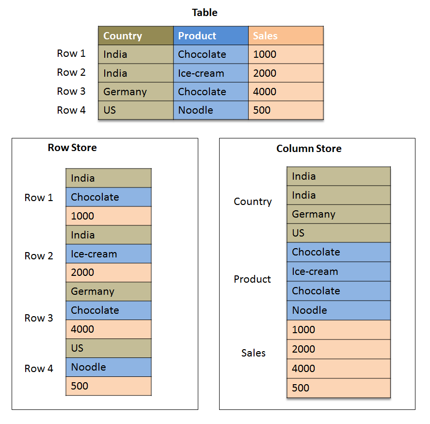
Source: SAP HANA Central
@task(name="Transform Data!")
def transform(data):
    for col in data.iloc[:, 1:].columns:
        data[col] = data[col].str.replace(r'[^0-9]+', '', regex=True).astype(int)
    return data
@task(name="Load Data!")
def load(data, path):
    data.to_parquet(path, compression='snappy')
When we have all the steps ready, we create a new function containing our graph using the flow decorator. We can give this function a name, for example, "Example Pipeline! 😎" and then chain the tasks we created previously in the order in which they should be run.
After we create our function, we can simply run it with the arguments necessary and Prefect will do its magic.
example_data_out = path.joinpath("example", "my_test.parquet")
type(example_data_out)
@flow(name="Example Pipeline! 😎")
def example_etl(example_data_in, example_data_out):
    data = extract(example_data_in)
    data_clean = transform(data)
    load(data_clean, example_data_out)
    print("Your Pipeline Ran Successfully!")
example_etl(example_data_in, example_data_out)#.execute_in_process()
To see the graph we just ran, we can open the terminal and run prefect orion start. This will take us to the Prefect UI where we can evaluate not only the run and graph, but also the parameters and logs collected from all DAGs we run.
To make sure we have the correct data, let's create a visualization with pandas and hvplot, a package that allows us to add interactivity to our pandas' charts.
import hvplot.pandas
pd.read_parquet(path.joinpath("example", "my_test.parquet")).hvplot(x='Year', y="ForestService")
6. 🐼 pipelines
The pipe operator is a pandas function that allows you to chain operations that take a data set, modify it, and return the modified version of the original data. In essence, it allows us to move the data through a series of steps until we reach the structure in which we want to have it.
For example, imagine that we have a group of data and 4 functions to fix it, the chain of operations would look like this.
(data.pipe(change_cols, list_of_cols)
     .pipe(clean_numeric_vars, list_of_numeric_vars)
     .pipe(add_dates_and_location, 'Auckland', 'NZ')
     .pipe(fix_and_drop, 'column_to_fix', seasons_NZ, cols_drop_NZ))
Another way to visualize what happens with pandas' pipe is through the following food process where we have ingredients and we actually require food.

Let's start with a small example without pipe first.
toy_data = pd.DataFrame({"Postal Codes": [22345, 32442, 20007],
                         "Cities":       ["Miami", "Dallas", "Washington"],
                         "Date":         pd.date_range(start='9/27/2021', periods=3)})
toy_data
def change_cols(data, cols_list):
    data.columns = cols_list
    return data
def clean_col_names(index_of_cols: pd.Index):
    import re
    new_cols =  [re.sub(r'[^a-zA-Z0-9\s]', '', col).lower().replace(r" ", "_") for col in index_of_cols]
    print(type(index_of_cols))
    print(index_of_cols)
    print(type(new_cols))
    print(new_cols)
pd.Index
clean_col_names(toy_data.columns)
change_cols(toy_data, ["postal_code", "city", "date"])
As you can see, with a single function it doesn't make much sense to pipe the process but with a chain of functions, the story changes.
The next thing we want to do is add additional information about the dates we have for each file. We can achieve this after converting the date variable to datetime format, which will allow us to access the year, month, week, ect. inside each date.
london_cols = ['date', 'count', 'temperature', 'temp_feels_like', 'humidity', 'wind_speed', 'weather_code', 'is_holiday', 'is_weekend', 'seasons']
seoul_cols = ['date', 'count', 'hour', 'temperature', 'humidity', 'wind_speed', 'visibility', 'dew_point_temp', 'solar_radiation', 'rainfall', 'snowfall', 'seasons', 'is_holiday', 'functioning_day']
wa_dc_cols = ['instant', 'date', 'seasons', 'year', 'month', 'hour', 'is_holiday', 'weekday', 'workingday', 'weathersit', 'temperature', 'temp_feels_like', 'humidity', 'wind_speed', 'casual', 'registered', 'count']
def add_dates_and_location(data, city, country):

    data['date']       = pd.to_datetime(data['date'], infer_datetime_format=True, dayfirst=True)
    data["year"]       = data['date'].dt.year
    data["month"]      = data['date'].dt.month
    data["week"]       = data['date'].dt.isocalendar().week.astype(int)
    data["day"]        = data['date'].dt.day
    data["weekday"]    = data['date'].dt.dayofweek
    data["is_weekend"] = (data["weekday"] > 4).astype(int)

    # note that we don't want to overwrite data that already has the hour as a column
    if 'hour' not in data.columns:
        data["hour"]   = data['date'].dt.hour
    data['date']       = data['date'].dt.date

    # non-date variables
    data['city']       = city
    data['country']    = country

    return data
add_dates_and_location(toy_data, "Sydney", "AU")
As you can see, we added a lot of information to our data with a simple function, but what happens when we want to chain two or three or four operations together? The following would not be very easy to read right?
add_dates_and_location(change_cols (toy_data, [" postal_code "," city "," date "])," Sydney "," AU ")
Let's move on to using our pipe operator now.
toy_data = pd.DataFrame({"Postal Codes": [22345, 32442, 20007],
                         "Cities":       ["Miami", "Dallas", "Washington"],
                         "Date":         pd.date_range(start='9/27/2021', periods=3)})
(
    toy_data.pipe(change_cols, ["zip_code", "city", "date"])
            .pipe(add_dates_and_location, "Sydney", "AU")
)
As you can see, now our chained functions are more readable than before and we can continue and chain even more functions in the same fashion.
In our data we have the stages of the year with different names and we also have variables that we do not need or that are not in the three files. Let's fix both!
seasons_london = {0: 'Spring', 1: 'Summer', 2: 'Fall', 3: 'Winter'}
seasons_wa_dc = {1: 'Spring', 2: 'Summer', 3: 'Fall', 4: 'Winter'}
holidays_seoul = {'No Holiday': 0, 'Holiday': 1}
cols_drop_london = ['temp_feels_like', 'weather_code']
cols_drop_seoul = ['visibility', 'dew_point_temp', 'solar_radiation', 'rainfall', 'snowfall', 'functioning_day']
cols_drop_wa_dc = ['instant', 'temp_feels_like', 'casual', 'registered', 'workingday', 'weathersit']
def fix_and_drop(data, col_to_fix, mapping, cols_to_drop):
    data[col_to_fix] = data[col_to_fix].map(mapping)
    return data.drop(cols_to_drop, axis=1)
Let's test the pipe operator but with the data from DC now and evaluate the results.
washington.head()
(washington.pipe(change_cols, wa_dc_cols)
           .pipe(fix_and_drop, 'seasons', seasons_wa_dc, cols_drop_wa_dc)).head()
Lastly, we esnt to create a function to normalize the data for DC as the columns are not in the same metric/imperial, etc. system as the rest.
def normalize_vars(data):
    data['temperature'] = data['temperature'].apply(lambda x: (x * 47) - 8)
    data['humidity']    = data['humidity'].apply(lambda x: (x / 100))
    data['wind_speed']  = data['wind_speed'].apply(lambda x: (x / 67))
    return data
Finally, we can use our pipe operator again to complete the process and see the end result.
Since we haven't created a function to read JSON files, let's create one anc call it extract_data.
def extract_data(path):
    return pd.read_json(path)
washington = (extract_data(wash_dc_path).pipe(change_cols, wa_dc_cols)
                                        .pipe(add_dates_and_location, 'DC', 'USA')
                                        .pipe(fix_and_drop, 'seasons', seasons_wa_dc, cols_drop_wa_dc)
                                        .pipe(normalize_vars))
washington.head()
Exercise
- Create a function to extract the London data.
- Create a data pipe similar to the one in Washington using pandas'
pipe.
7. Extract
Depending on where the data is, in what format it is stored, and how we can access it, this can either be one of the shortest steps or one of the longest ones in our data pipeline. Here are some of the formats that you might encounter in your day to day.
- Text: usually the text format is similar to what we see in Microsoft Excel but without formulas or graphics. For example, CVS or TSV.
- JSON: JavaScript Object Notation is a very popular sub-language for its simple syntactics
- Databases: These can be SQL, NOSQL, MPP (massively parallel processing), among others.
- GeoJSON: It is a type of format for data that contains geographic information. There are many more types of data for GIS.
- HTML: Refers to Hyper Text Markup Language and represents the skeleton of almost all web pages in existence.
- ...
Since we already learned how to create useful pipelines with pandas, we now need to create functions for our main ETL pipeline to automate the process. We can achieve this using the prefect decorator, @task from earlier. This decorator takes note of the functions that we want to link together and helps us create a network in which each node is a function and each link connects one or more functions only once.
Remember, the decorator @task is also a function within prefect and as such, we can pass several arguments to it that help us modify the behavior of each function in our pipeline.
You can learn more about the task API in the official docs here.
task??
@task
def extract_1(path):
    return pd.read_csv(path)
@task
def extract_2(path):
    conn = sqlite3.connect(path)
    query = "SELECT * FROM uk_bikes"
    return pd.read_sql_query(query, conn)
@task
def extract_3(path):
    return pd.read_json(path)
8. Transform
The most common transformations that happen at this stage are usually the ones we created earlier. In short,
- Clean text data
- Normalize columns
- Convert numeric variables to the same unit
- Deal with missing values
- Join data
Our transform step will be a parent function to our pipe operators from earlier. Hence, a combination of functions handle by a single one.
def order_and_merge(data_lists):

    pick_order = data_lists[0].columns
    new_list = [d.reindex(columns=pick_order).sort_values(['date', 'hour']) for d in data_lists]
    df = pd.concat(new_list)
    return df
@task
def transform(london, seoul, washington):

    london = (london.pipe(change_cols, london_cols)
                    .pipe(add_dates_and_location, 'London', 'UK')
                    .pipe(fix_and_drop, 'seasons', seasons_london, cols_drop_london))

    seoul = (seoul.pipe(change_cols, seoul_cols)
                  .pipe(add_dates_and_location, 'Seoul', 'SK')
                  .pipe(fix_and_drop, 'is_holiday', holidays_seoul, cols_drop_seoul))

    wash_dc = (washington.pipe(change_cols, wa_dc_cols)
                         .pipe(add_dates_and_location, 'DC', 'USA')
                         .pipe(fix_and_drop, 'seasons', seasons_wa_dc, cols_drop_wa_dc)
                         .pipe(normalize_vars))

    return order_and_merge([london, seoul, wash_dc])
9. Load
We will need to save our new file in a database or in a format in which we are given both what the file occupies and the speed with which we can open and use it. So we will create two paths and two names for the files that we will use later.
clean_path = path/'processed/clean.parquet'
clean_db_path = path/'processed/bikes'
clean_db_path
We will have a function for saving the data in a database. For this, Prefect provides us with a wrapper function around SQLite called, SQLiteScript which allows us to create a database and run a SQL scipt on top of it. This comes in hady for large and small operations/prototypes alike.
def SQLiteScript(db, script):
    with closing(sqlite3.connect(db)) as conn:
        with closing(conn.cursor()) as cursor:
            cursor.executescript(script)
script= """
            CREATE TABLE IF NOT EXISTS bike_sharing (
                    date text, count integer, temperature real,
                    humidity real, wind_speed real, is_holiday real,
                    is_weekend integer, seasons text, year integer,
                    month integer, week integer, day integer,
                    hour integer, weekday integer, city text,
                  country text
              )
"""
next(washington.itertuples(name='Bikes', index=False))
@task
def load(data, path_and_name):

    data = list(data.itertuples(name='Bikes', index=False))

    insert_cmd = "INSERT INTO bike_sharing VALUES (?, ?, ?, ?, ?, ?, ?, ?, ?, ?, ?, ?, ?, ?, ?, ?)"
    with closing(sqlite3.connect(path_and_name)) as conn:
        with closing(conn.cursor()) as cursor:
            cursor.executemany(insert_cmd, data)
            conn.commit()
10. Launch a Pipeline
In the same fashion as before, we will combine our functions in a function decorated with flow to signal to prefec's scheduler that we have a DAG we would like to run.
@flow(name='bikes-ETL')
def my_etl():

    new_table = SQLiteScript(db=str(clean_db_path), script=script)

    london = extract_2(london_path)
    seoul = extract_1(seoul_path)
    wash_dc = extract_3(wash_dc_path)

    transformed = transform(london, seoul, wash_dc)

    data_loaded = load(transformed, clean_db_path)
Running our pipeline is as simple as calling the function. In addition, even though we did not pass in any parameters to our flow function, it can contain any number of them if we choose to.
my_etl()
pd.read_sql_query("SELECT * FROM bike_sharing", sqlite3.connect(clean_db_path)).head()
Exercise
Change the function to unload (load ()) and make it save the results in parquet format. Run the pipeline again and make sure the results are the same as above by reading the data with pandas' respective function for parquet files.
11. Summary
- Creating ETL pipes helps us automate the cleaning steps to prepare our datasets.
- pandas
pipehelps you chain functions that operate on a dataframe and return a dataframe, effectively helping us save time and lines of code. - Prefect helps us create, monitor, and schedule directed acyclic graphs represented via the steps of our cleaning process.