Data Pipelines From Scratch
“Without a systematic way to start and keep data clean, bad data will happen.” ~ Donato Diorio
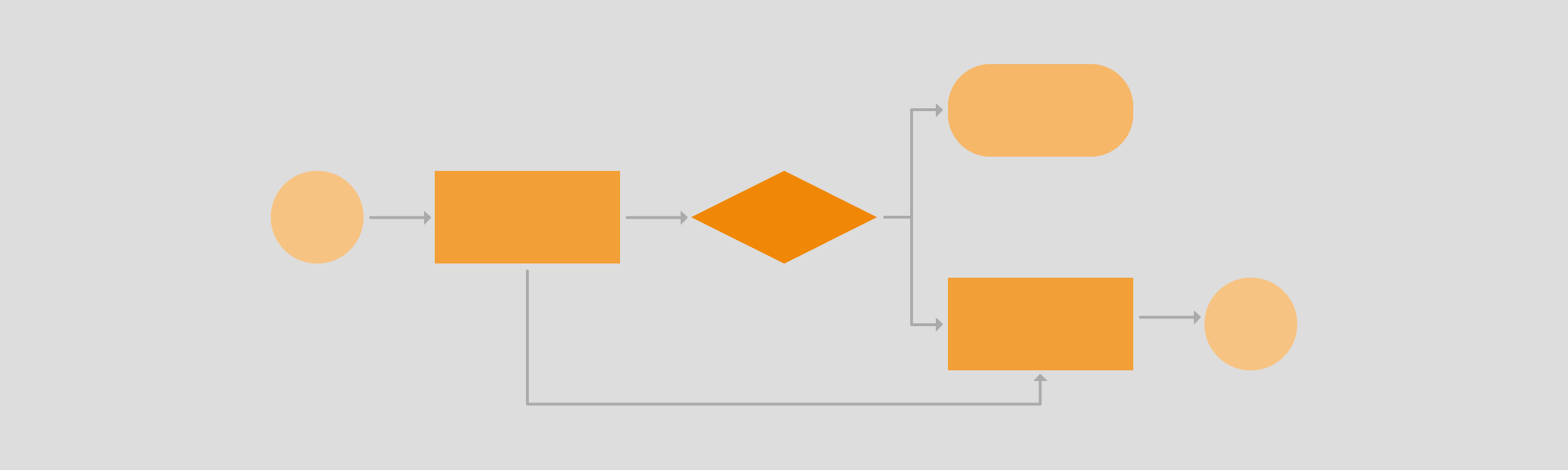
Source: draw.io
Table of Contents
- Overview
- Learning Outcomes
- Data
- Tools
- Data Pipelines
- Building a Framework
- Set Up Dev Environment
- Extract
- Transform
- Load
- Reproducible Pipelines
- Scheduling
- Exercises
- Resources
1. Overview
In order to create successful and reproducible data pipelines we need -- at the bare minimum -- tools that allow us manage where and how we store our data, how we run our computations, and how we version control everything we do. This is what we will focus on in this part of the workshop.
The assumption of this section is that most of your data work can fit in a computer but, if the need were to arise, you could still use the code in this section with a beefier machine and it would get the job done without a problem.
Since the files we'll interact with will most likely live in a remote server, we'll
- extract a copy of the data we'll use and save it to our local files;
- transform the data into the shape and form we need it to be in;
- load it into a local data warehouse based on the popular tool, duckdb;
- version our code and data using dvc and git;
- create a command line tool to run all of our jobs;
- create a reproducible pipeline that can capture different workflows.
Before we get started, let's go over the learning outcomes for today. :)
Note: While one of the main components of data orchestration is scheduling, you can sill create pipelines and reproducible workflows that can be triggered manually rather than via a schedule.
2. Learning Outcomes
Before we get started, let's go over the learning outcomes for this section of the workshop.
By the end of this lesson you will be able to,
- Discuss what ETL and ELT Pipelines are.
- Understand how to read and combine data that comes from different sources.
- Create data pipelines using open-source tools.
- Develop command line tools.
3. Data

All three data files contain similar information about how many bicycles have been rented each hour, day, week and months for several years and for each city government we are working with.
You can get more information about the data of each city using the following links.
- Seoul, South Korea
- London, England, UK
- Washington, DC, USA
- Porto, Portugal -- This one was shared in Kaggle, but you can also find the original source with more, up-to-date data, here.
Note: Some datasets might come with another file containing daily information, but for our purposes, we will be using the hourly one.
Here are the variables that appear in all data sets.
| London | Seoul | Washington | Porto |
|---|---|---|---|
| date | Date | instant | instant |
| count | Rented Bike Count | date | dteday |
| temperature | Hour | seasons | season |
| t2 | Temperature(C) | year | yr |
| humidity | Humidity(%) | month | mnth |
| wind_speed | Wind speed (m/s) | hour | hr |
| weather_code | Visibility (10m) | is_holiday | holiday |
| is_holiday | Dew point temperature(�C) | weekday | weekday |
| is_weekend | Solar Radiation (MJ/m2) | workingday | workingday |
| seasons | Rainfall(mm) | weathersit | weathersit |
| Snowfall(cm) | temperature | temp | |
| Seasons | count | atemp | |
| Holiday | humidity | hum | |
| Functioning Day | wind_speed | windspeed | |
| casual | casual | ||
| registered | registered | ||
| cnt |
Since all of these datasets were generated with different logic (e.g. celsius vs fahrenheit, or other divergent measures) and, most likely, by different systems, we can expect more inconsistencies than just unmatching column names, numerical formats, and data collected.
We will walk through an example pipeline and several cleaning steps after we discuss the tools we will be using today.
4. Tools
The tools that we will use in this section of the workshop are the following.
- pandas - "is a fast, powerful, flexible and easy to use open source data analysis and manipulation tool, built on top of the Python programming language."
- dvc - "DVC is built to make ML models shareable and reproducible. It is designed to handle large files, data sets, machine learning models, and metrics as well as code."
- ibis - "Ibis is a Python library that provides a lightweight, universal interface for data wrangling. It helps Python users explore and transform data of any size, stored anywhere."
- typer - "Typer is a library for building CLI applications that users will love using and developers will love creating. Based on Python 3.6+ type hints."
- pathlib - allows us to manipulate paths as if they were python objects.
Let's get started building data pipelines! :)
5. Data Pipelines
Source: Striim
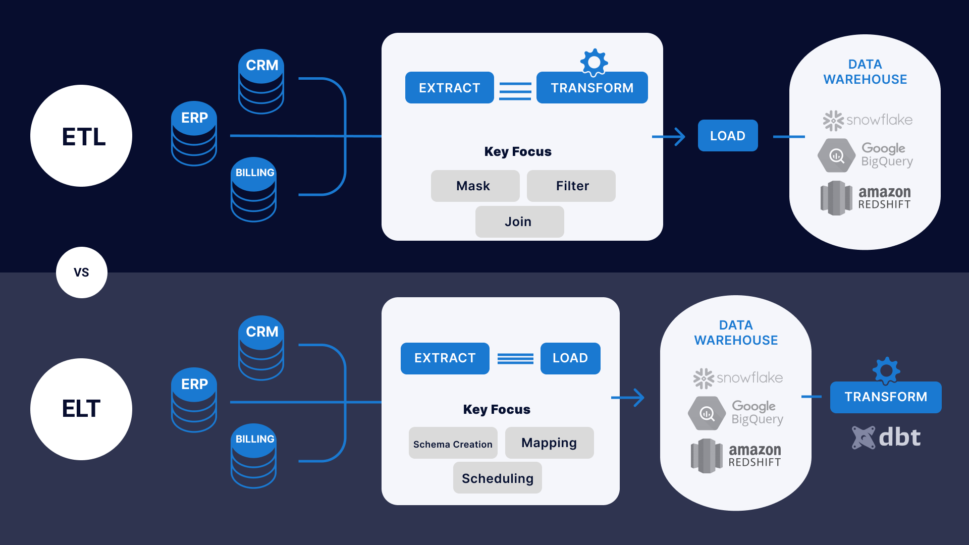
There are different kinds of data pipelines, but two, in particular, dominate a big part of the data engineering world today, ETL and ELT pipelines.
What are ETL Pipelines?
The acronym ETL stands for Extract, Transform, and Load, and it is the process where data gets extracted from one or multiple sources, it gets processed in-transit, and then it gets loaded into place where data consumers can use (e.g. a data warehouse). These consumers can be data analysts, data scientists, and machine learning engineers, among many others.
What are ELT Pipelines? With this approach, all the data, structured and unstructured, gets loaded into a data lake or warehouse before it gets transformed. With this approach, a lot of money spent on compute can be saved by only processing the data we need rather than all of it.
What are Reverse ETL Pipelines? Reverse ETL tools take data from the data lake or warehouse back into business (critical) applications. For example, information about new customers that have not yet been populated into salesforce or other marketing tools for further use by the marketing, sales, and finance teams, and so on...
Why should you learn how to create them?
Data Pipeline tools enable data integration strategies by allowing companies to gather data from multiple data sources and consolidate it into a single, centralized location. ETL tools also make it possible for different types of data to work together, for example, data generated by the company can be combined with GPS and Temperature data coming from different sources.
As data professionals, our task is to create value for our organizations, our clients and our collaborators using some of or all the data at our disposal. However, there are factors that can delay this process a little bit or a lot, for example, we often need to understand beforehand,
- Information about the process by which the data we're dealing with was generated, e.g.
- Point of sale
- Clicks on an online marketplace like Amazon, Etzy, Ebay, ect.
- A/B Test Results
- ...
- Information about the transformations that occurred during the cleaning and merging process, prior to us jumping on board,
- Celsius degrees were converted into fahrenheit
- Prices in Chilean pesos were converted to Rands
- Non-numerical and unavailable observations now contain "Not Available" or "Unknown"
- ...
- Information about how the data was stored and where. For instance,
- Parquet format
- NOSQL or SQL database
- CSV
- ...
Understanding how the three processes described above flow will help us have more knowledge about the data that we are going to use, and how to best access it, transform it, and model it before we put it to good use.
Let's walk through an example of a data pipeline using data from wildfires between 1983-2020 in the United States. You can find more information about the dataset here.
import pandas as pd
from pathlib import Path
!pwd
data_path = Path().cwd().parent/"data"
data_path
example_data_in = data_path.joinpath("example", "federal_firefighting_costs.csv")
pd.read_csv(example_data_in).head()
pd.read_csv(example_data_in).dtypes
As you can see, most columns contain a $ dollar sign and some , commas, and because this forces Python to treat numbers as objects (or strings) rather than int's or float's, we will have to remove these signs in our transformation step after extracting the data and before loading a clean version of it to a new location. Let's create 3 re-usable functions.
def extract(path):
    return pd.read_csv(path)
As you saw above, only the last 5 variables have commas (,) and dollar symbols ($) so we will replace both with an empty space ("") using a for loop.
def transform(data):
    for col in data.iloc[:, 1:].columns:
        data[col] = data[col].str.replace(r'[^0-9]+', '', regex=True).astype(int)
    return data
For the "load" process, we will save the data as a parquet file. This is one of the most popular formats to save data in due to its compression capabilities, orientation, and speed gains in analytical workloads.
Here's an example on the differences between the row-like format and the columnar format of parquet files. If this interests you you can read more about it here
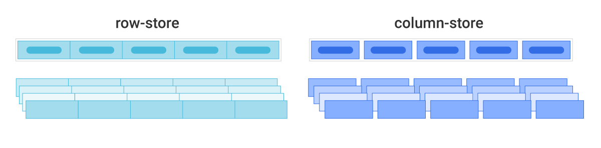
Source: Scylla DB
def load(data, path):
    data.to_parquet(path)
    print("Successfully Loaded Your Modified Data!")
Let's create an output path and with a file name to save our data as.
data_path
example_data_out = data_path.joinpath("example", "my_test.parquet")
When we have all the steps ready, we create a new function containing our graph using the flow decorator. We can give this function a name, for example, "Example Pipeline! 😎" and then chain the tasks we created previously in the order in which they should be run.
def example_etl(example_data_in, example_data_out):
    data = extract(example_data_in)
    data_clean = transform(data)
    load(data_clean, example_data_out)
    print("Your Pipeline Ran Successfully!")
We are ready to run our workflow.
example_etl(example_data_in, example_data_out)
To make sure we did everything correctly, let's create a quick visualization with pandas.
pd.read_parquet(example_data_out).plot(
    x='Year',
    y="ForestService",
    kind='line',
    title="Forest Service costs by year"
);
6. Building a Framework
In order to do our data engineering work with a personalized framework, there are a few strategies we would take.
- We could keep the code in our computers and copy it to a new project whenever we need to create new pipelines.
- We could create a package and either upload it to PyPI or Gemfury (a private repository of packages for different programming languages).
- We could keep in neatly organized in GitHub and clone the repository to every new project.
For this use case, it would be great to work with a library that we could continuously update rather than notebooks and files getting copied around. This will help us stay organized and manage dependencies more effectively.
Let's get started. :)
6.1 Setting Up a Dev Environment
Building frameworks can be super straightforward or a slightly cumbersome project. Because of this and because we are already using an environment to run this workshop in, I will leave here what I think is an excellent resource for learning about how to create Python Packages.
from IPython.display import HTML
HTML("""
<div align="center">
    <iframe width="700" height="450"
    src="https://youtube.com/embed/l7zS8Ld4_iA"
    </iframe>
</div>
""")
6.2 Extract
Extracting data might seem straightforward, but it can come with plenty of caveats. For example, to access sensitive data you might need not only credentials but also access to VPNs (virtual private networks), you might have similar data in different kinds of formats (customer tables stored in legacy databases and new ones), or you might have different data all stored in one place (images, tables, and text all in a datalake) -- if you're lucky.
To tackle these challenges, (1) access and (2) distribution of data, companies such as Airbyte, Fivetran, and others, have come up with solutions that do all the heavy lifting for us. They have created tools that either give you connectors to common data sources (such as S3, BigQuery, and others), or give you an API so that you can develop a custom connector.
That said, what we'll do in this section is to create functions that allow us to extract data in different formats or download a dataset from the web. We will create one for each of the examples that we have for the workshop today. Let's get started loading some data.
import urllib.request
def get_and_load_file(url, path_out, file_name):
    path = Path(path_out)
    if not path.exists(): path.mkdir(parents=True)
    urllib.request.urlretrieve(url, path.joinpath(file_name))
get_and_load_file(
    url="https://archive.ics.uci.edu/ml/machine-learning-databases/00560/SeoulBikeData.csv",
    path_out="../data/example",
    file_name="seoul_exp.csv"
)
The function above will download the file into the "data/example" directory. If we do not specify a path for the file to urllib.request.urlretrieve, it would download the file into a temporary directory since it wouldn't know what to do with it or where to put it.
A popular alternative to urllib is wget, so you can switch the tools in this function easily. The former is part of the Python Standard Library (so you'll never have to install it), and the latter can be installed with pip or conda.
Let's create two more, one for csv files and the other for parquet files.
def extract_from_csv(path_in, encoding=None):
    return pd.read_csv(path_in, encoding=encoding)
seoul_df = extract_from_csv(
    path_in=data_path.joinpath("seoul", "raw", "SeoulBikeData.csv")
)
seoul_df.head()
The reason, we've added enconing to our function is that files are not always shared in utf-8 abd it is important to account for this discrepancy when creating an ETL framework. In fact, one of our datasets has a tricky format itself.
{1: "value", 1: "value", 1: "value", 1: "value", }
def extract_from_parquet(path_in, **kwargs):
    return pd.read_parquet(path_in, **kwargs)
porto_df = extract_from_parquet(
    path_in=data_path.joinpath("porto", "bike_sharing_hourly.parquet")
)
porto_df.head()
One of our files is stored in a SQLite database so we'll use the sqlite3 module, which is part of of the Python Standard Library, to read it.
import sqlite3
def extract_from_db(path_in, query):
    conn = sqlite3.connect(path_in)
    return pd.read_sql_query(query, conn)
london_df = extract_from_db(
    path_in=data_path.joinpath("london", "london_bikes.db"),
    query="SELECT * FROM uk_bikes"
)
london_df.head()
Lastly, JSON files can be tricky to handle so we'll try two quick cases here using a try-except approach, but take note that as your projects evolve, it is highly likely that this function might change. A very good tool to handle large amounts of unstructured JSON that can later be formatted as a dataframe (or many), is Dask Bags.
def extract_from_json(path_in, **kwargs):
    try:
        data =  pd.read_json(path_in, kwargs)
    except:
        with open(path_in, 'r') as f:
            data = json.loads(f.read())
            data = pd.json_normalize(data, kwargs)
    return data
dc_df = extract_from_json(
    path_in=data_path.joinpath("wash_dc", "washington.json")
)
dc_df.head()
Now that we have our functions, we want to create a file and attach to it the minimum functionality possible to use it as a command line tool. We will do this with the popular package called typer. It offers a delightful user experience, it respects (and annoys you at times) by type-checking your code, and it provides you with beautifully-formatted output based on the rich python library.
With typer we can create CLIs in several ways, and, for our purposes, we will pick the most straightforward one which works by adding typer.run() around a main function that encapsulates your application logic, in our case, our extract function and the upcoming ones.
%%writefile ../src/data_eng/extract.py

import urllib.request
from pathlib import Path
import pandas as pd
import json
import typer
from typing import Optional
from load import save_data


def get_and_load_file(url, path_out, file_name):
    path = Path(path_out)
    if not path.exists():
        path.mkdir(parents=True)
    urllib.request.urlretrieve(url, path.joinpath(file_name))

def extract_from_csv(path_in, encoding=None):
    return pd.read_csv(path_in, encoding=encoding)

def extract_from_db(path_in, query):
    conn = sqlite3.connect(path_in)
    return pd.read_sql_query(query, conn)

def extract_from_parquet(path_in, **kwargs):
    return pd.read_parquet(path_in, **kwargs)

def extract_from_json(path_in, **kwargs):
    try:
        data =  pd.read_json(path_in, **kwargs)
    except:
        with open(path_in, 'r') as f:
            data = json.loads(f.read())
            data = pd.json_normalize(data, kwargs)
    return data

def main(
    arg: str = typer.Option(...),
    url: Optional[str] = typer.Option(None),
    path_in: Optional[str] = typer.Option(None),
    path_out: Optional[str] = typer.Option(None),
    encoding: Optional[str] = typer.Option(None),
    file_name: Optional[str] = typer.Option(None),
    query: Optional[str] = typer.Option(None),
):
    if arg == "get":
        get_and_load_file(url, path_out, file_name)
    elif arg == "csv":
        data = extract_from_csv(path_in, encoding=encoding)
        save_data(data, path_out, file_name)
    elif arg == "pq":
        data = extract_from_parquet(path_in)
        save_data(data, path_out, file_name)
    elif arg == "json":
        data = extract_from_json(path_in)
        save_data(data, path_out, file_name)
    elif arg == "db":
        data = extract_from_db(path_in, query)
        save_data(data, path_out, file_name)
    else:
        print(f"Could not understand argument {arg}. Please use 'pq' for parquet files, 'db' for database, json, or csv in lowercase.")

    print("Data Extracted Successfully!")


if __name__ == "__main__":
    typer.run(main)
Note that we added different parameters to our main function to control the behavior of our CLI app.
arg- the kind of data we're extracting.url- the url for when we need to download files from somewherepath_in- where is the data atpath_out- where is that data going toencoding- what kind of enconding are we reading the file withfile_name- what is going to be the new name of the output filequery- query for the data we want from the SQL database
A few important things to note:
- parameters containing underscores
_will be switched into a dash-bytyper, sofile_namewill befile-name - commands are run with two dashes and with a space in between it and the argument being passes, e.g.
--name PyCon typer.Option(None)indicates totyperthat this command can be optional, hence, when we change the kind of file we're extracting we can by pass having to put an option on others.- by adding
Optionalaround the type of a function parameter, you are also letting typer that that parameter is optional and that its default argument isNone. - a parameter with only a type is a required parameter.
pd.read_parquet("../data/seoul/raw/testing_cli_extract2.csv").head()
6.3 Transform
Depending on tasks that await the final output files or tables of an ETL pipeline (e.g. reporting metrics, building machine learning models, forecasting, etc.), this step can be very convoluted or slightly straightforward. In general, though, this step can include lots of cleaning and normalization functions, and a schema setter, among many others.
The cleaning steps might include dealing with missing values, cleaning emails, names, addresses, and others, or putting values of similar nature into the same format (e.g. different weather measurements into one).
Normalization can be anything from changing column names with the same values but different names to have the same one, or height in cm vs feet and inches to be in the same measure, or ..., you get the point. :)
A schema is the way in which we represent not only the content and type of our new data files/tables, but also the way in which we represent their relationship. A common schema is the star schema. An uncommon (but rising star) schema is the activity schema.
import re
#create some toy data for our Bicycle problem

toy_data = pd.DataFrame({"Postal Codes": [22345, 32442, 20007],
                         "Cities'":       ["Miami,  FL", "Dallas, TX", "Washington, DC"],
                         "Dates as mm-dd-yyy":         pd.date_range(start='9/27/2021', periods=3)})
toy_data
def clean_col_names(index_of_cols: pd.Index):
    return [re.sub(r'[^a-zA-Z0-9\s_]', '', col).lower().replace(r" ", "_") for col in index_of_cols]
clean_col_names(toy_data)
def extract_dates(data, date_col, hour_col=None):

    data["date"] = pd.to_datetime(data[date_col], infer_datetime_format=True)
    if not data.columns.isin(["hour", "Hour", "hr", "HR"]).any():
        data["hour"] = data['date'].dt.hour
        #Time series datasets need to be ordered by time.
        data.sort_values(["date", "hour"], inplace=True)
    elif hour_col:
        data.sort_values(["date", hour_col], inplace=True)
    else:
        print("You must figure out how the hour works in your file.")

    data["year"]           = data['date'].dt.year
    data["month"]          = data['date'].dt.month
    data["week"]           = data['date'].dt.isocalendar().week
    data["day"]            = data['date'].dt.day
    data["day_of_week"]    = data['date'].dt.dayofweek
    data["is_month_start"] = data['date'].dt.is_month_start

    data.drop('date', axis=1, inplace=True)
    return data
extract_dates(london_df, "timestamp").head()
A common tasks in data science is to create dummy variables, which is ofter referred to as one-hot encoding. These are binary representations of a category, for example, if you have a columns with different kinds of cars, after you one-hot encode it, you will have one column for sedan, coupe, convertible, and so on, and each will be represented with a 0 or a 1 for when it is available and when it isn't, respectively.
def one_hot(data, cols_list, **kwargs):
    return pd.get_dummies(data=data, columns=cols_list, **kwargs)
one_hot(seoul_df, ["Seasons", "Holiday"], drop_first=True).head()
def add_location_cols(data, place):
    data["loc_id"] = place
    return data
add_location_cols(dc_df, "DC").head()
def fix_and_drop(data, col_to_fix, mapping, cols_to_drop):
    data[col_to_fix] = data[col_to_fix].map(mapping)
    return data.drop(cols_to_drop, axis=1)
seasons_london = {'Spring': 0, 'Summer': 1, 'Fall': 2, 'Winter': 3}
cols_drop_london = ['t2', 'weather_code']
london_df.head()
london_df["seasonreal"].map(seasons_london).value_counts()
fix_and_drop(london_df, "seasonreal", seasons_london, cols_drop_london).head()
def order_and_merge(data_lists, date=None):
    pick_order = data_lists[0].columns #takes order of columns of the first dataset
    #reindexing columns by the order of the first dataset, then sorting by date and hour.
    if date:
        new_list = [d.reindex(columns=pick_order).sort_values([date, 'hour']) for d in data_lists]
    else:
        new_list = data_lists
    return pd.concat(new_list) #merge all
Exercise
Pick any two datasets and
- select 5 columns from each
- change column names as appropriate
- use the order_and_nerge function to combine both
london_df.head()
london_df_small = london_df[["cnt", "t1", "wind_speed", "seasonreal", "hour"]]
london_df_small.tail()
seoul_df.head()
seoul_df_small = seoul_df[["Rented Bike Count", "Temperature(�C)", "Wind speed (m/s)", "Seasons", "Hour"]]
seoul_df_small.head()
seoul_df_small.columns = london_df_small.columns
seoul_df_small.columns == london_df_small.columns
order_and_merge([seoul_df_small, london_df_small]).shape
Finally, we take the same approach as with the extract set of functions and wrap our transform workflow into a main function, and then that main function into a typer CLI.
%%writefile ../src/data_eng/transform.py

import pandas as pd, re
from pathlib import Path
from extract import save_data
import typer
from typing import Optional, List

def clean_col_names(index_of_cols: pd.Index):
    return [re.sub(r'[^a-zA-Z0-9\s_]', '', col).lower().replace(r" ", "_") for col in index_of_cols]

def extract_dates(data, date_col, hour_col=None):

    data["date"] = pd.to_datetime(data[date_col], infer_datetime_format=True)
    if not data.columns.isin(["hour", "Hour", "hr", "HR"]).any():
        data["hour"] = data['date'].dt.hour
        #Time series datasets need to be ordered by time.
        data.sort_values(["date", "hour"], inplace=True)
    elif hour_col:
        data.sort_values(["date", hour_col], inplace=True)
    else:
        print("You must figure out how the hour works in your file.")

    data["year"]           = data['date'].dt.year
    data["month"]          = data['date'].dt.month
    data["week"]           = data['date'].dt.isocalendar().week
    data["day"]            = data['date'].dt.day
    data["day_of_week"]    = data['date'].dt.dayofweek
    data["is_month_start"] = data['date'].dt.is_month_start

    data.drop('date', axis=1, inplace=True)
    return data

def one_hot(data, cols_list):
    return pd.get_dummies(data=data, columns=cols_list)

def add_location_cols(data, place):
    data["loc_id"] = place
    return data

def fix_and_drop(data, col_to_fix, mapping, cols_to_drop):
    data[col_to_fix] = data[col_to_fix].map(mapping)
    return data.drop(cols_to_drop, axis=1)

def order_and_merge(data_lists):
    pick_order = data_lists[0].columns #takes order of columns of the first dataset
    new_list = [d.reindex(columns=pick_order).sort_values(['date', 'hour']) for d in data_lists] #reindexing columns by the order of the first dataset, then sorting by date and hour.
    return pd.concat(new_list) #merge all

def main(
    path_in:   str           = typer.Option(...),
    date_col:  Optional[str] = typer.Option(None),
    hour_col:  Optional[str] = typer.Option(None),
    cols_list: List[str]     = typer.Option(None),
    place:     Optional[str] = typer.Option(None),
    path_out:  Optional[str] = typer.Option(None),
    file_name: Optional[str] = typer.Option(None)
):
    data = pd.read_parquet(path_in)
    # data.columns = clean_col_names(data.columns)
    data = extract_dates(data, date_col, hour_col)
    if cols_list:
        data = one_hot(data, cols_list)
    data.columns = clean_col_names(data.columns)
    data = add_location_cols(data, place)
    save_data(data, path_out, file_name)

    print("Data Extracted and Transformed Successfully!")

if __name__ == "__main__":
    typer.run(main)
pd.read_parquet("../data/seoul/interim/cli_test_clean.parquet").head()
6.2 Load
The loading stage, at least for analytical purposes, tends to be a data warehouse like BigQuery, Redshift, etc., but it can also be a directory in a data lake where files are saved in the highly optimized parquet format.
In order for us to simulate a data warehouse locally, we will create a duckdb database using the python library ibis. The reason we will do it this ways is that ibis can translate the schema of our files into the duckdb SQL in one line of code. Effectively saving us boilerplate code that may or may not end up accounting for every feature in our dataframes.
Ibis is a very cool project, especially if your SQL skills as basic as mine, so I highly encourage you to check it out. :)
import ibis
from pathlib import Path
data_path = Path().cwd().parent/"data/"
def create_db(path_in, path_out, file_name, table_name):
    path = Path(path_out)
    conn = ibis.duckdb.connect(path.joinpath(file_name))
    conn.register(path_in, table_name=table_name)
    print(f"Successfully loaded the {table_name} table!")
create_db(
    path_in=data_path.joinpath("porto", "bike_sharing_hourly.parquet"),
    path_out="../data/dwarehouse",
    file_name="mytest_dw.ddb",
    table_name="one_day"
)
Let's read in our data to check that it was loaded successfully.
import duckdb
duck = duckdb.connect("../data/dwarehouse/mytest_dw.ddb")
duck.query("SELECT * FROM one_day").df().head()
def create_parquet(path_in, path_out, file_name):
    path = Path(path_out)
    pd.read_parquet(path_in).to_parquet(path.joinpath(file_name))
    print(f"Successfully loaded the {file_name} table!")
def save_data(data, path_out, file_name):
    path_out = Path(path_out)
    if not path_out.exists(): path_out.mkdir(parents=True)
    data.to_parquet(path_out.joinpath(file_name))
    print(f"Successfully loaded the {file_name} table!")
We take the same steps as before and wrap our main function with typer.run() to make it a CLI, we test that it works well, and then go on to the next stage.
%%writefile ../src/data_eng/load.py

from pathlib import Path
import ibis
import typer
from typing import Optional
import pandas as pd


def create_db(path_in, path_out, file_name, table_name):
    path = Path(path_out)
    conn = ibis.duckdb.connect(path.joinpath(file_name))
    conn.register(path_in, table_name=table_name)
    print(f"Successfully loaded the {table_name} table!")

def create_parquet(path_in, path_out, file_name):
    path = Path(path_out)
    pd.read_parquet(path_in).to_parquet(path.joinpath(file_name))
    print(f"Successfully loaded the {file_name} table!")

def save_data(data, path_out, file_name):
    path_out = Path(path_out)
    if not path_out.exists(): path_out.mkdir(parents=True)
    data.to_parquet(path_out.joinpath(file_name))
    print(f"Successfully loaded the {file_name} table!")


def main(
    kind: str = typer.Option(...),
    path_in: Optional[str] = typer.Option(None),
    path_out: Optional[str] = typer.Option(None),
    file_name: Optional[str] = typer.Option(None),
    table_name: Optional[str] = typer.Option(None)
):
    if kind == "db":
        create_db(path_in, path_out, file_name, table_name)
    elif kind == "pq":
        create_parquet(path_in, path_out, file_name)
    else:
        print(f"Could not understand argument {kind}. Please use 'pq' for parquet files or 'db' for database.")

    print("Data Extracted Successfully!")

if __name__ == "__main__":
    typer.run(main)
7. Reproducible Pipelines
Data Version Control or dvc is a tool for version almost any kind of file you can think of. From images, text, videos, and excel spreadsheets, to machine learning models and other artifacts. In addition, it is also an excellent tool for tracking machine learning experiments and for creating language agnostic pipelines where you can automatically version control the inputs and outputs of your workflows.
If you have ever used git then the following commands will feel like home
dvc init--> this the first step to get started using dvc (after installing it of course)dvc remote add -d storage gdrive://your_hash--> since we will be tracking files somewhere, this command will help set up a remote repository for these.dvc add--> add a file to track.dvc push--> push the file to your remote repository.dvc pull--> pull the file from your remote repository and into your local machine.dvc stage--> allows you to start adding steps to a pipeline. It will create advc.ymlfile containing the steps of the pipeline. This can be modified manually as well.dvc repro--> Once we finish our stage, or as we add steps to it, we can run our pipeline with this command. The best part is that the steps will get cashed, so if nothing changes, nothing will get rerun.dvc dag--> allows you to visualize your pipelines as a graph in the terminal.
Finally, some of the settings for our repo will be available at .dvc/config and these can be changed manually at any time.
Open a terminal in the main directory for this workshop and follow along.
To create our pipeline, we'll add the stages step by step.
dvc stage add --name seoul_extract \
    --deps data/seoul/SeoulBikeData.csv \
    --outs data/seoul/raw/seoul_raw.parquet \
    python src/data_eng/extract.py --arg csv \
        --path-in data/seoul/SeoulBikeData.csv \
        --path-out data/seoul/raw \
        --file-name seoul_raw.parquet --encoding iso-8859-1
dvc stage add --name seoul_transform \
    --deps data/seoul/raw/seoul_raw.parquet \
    --outs data/seoul/interim/seoul_clean.parquet \
    python src/data_eng/transform.py \
        --path-in data/seoul/seoul_raw.parquet \
        --date-col Date --hour-col Hour --place Seoul \
        --path-out data/seoul/interim --file-name seoul_clean.parquet
Exercise
Add the load stage into our pipeline following the examples above.
dvc stage add --name seoul_load \
    --deps data/seoul/interim/seoul_clean.parquet \
    --outs data/dwarehouse/analytics.db \
    python src/data_eng/load.py --kind db \
        --path-in data/seoul/interim/seoul_clean.parquet \
        --path-out data/dwarehouse --name analytics.db \
        --table-name seoul_main
Finally we can run our pipeline, evaluate it, and push our files into our remote storage.
# 1
dvc repro

# 2
dvc dag

# 3
dvc push
Afterwards, dvc will provide us with git files to track for our project.
8. Scheduling
Scheduling our workflows can be super convenient and time-savior when we know we need to run tasks repeatedly. A very common tool for the task is cron, and here is an excellent tutorial to get started with it.
Note: Windows users would need to use Windows Subsystem for Linux to use cron or some other tool, potentially in PowerShell.
from IPython.display import HTML
HTML("""
<div align="center">
    <iframe width="700" height="450"
    src="https://www.youtube.com/embed/QZJ1drMQz1A"
    title="YouTube video player" frameborder="0" allow="accelerometer; autoplay;
    clipboard-write; encrypted-media; gyroscope; picture-in-picture;
    web-share" allowfullscreen>
    </iframe>
</div>
""")
9. Exercises
Exercise 1
- Open the terminal, create a new directory named
dc_bikes, and cd into it. - Create two subdirectories, data and src.
- Create an ETL pipeline with two functions in the transform step.
Exercise 2
- Initialize a git and a dvc repository for the project in Exercise 1.
- Create a new repo in GitHub and commit your initial changes.
- Create a dvc pipeline with your three stages.
- Commit your changes.
10. Resources
If you'd like to expand your knowledge around the tools and concepts that we covered in this lesson, you might find the following list of resources helpful.
- To learn more about pandas --> Python for Data Analysis, 3E by Wes McKinney
- To learn more about ibis --> Ibis + Substrait + DuckDB by Gil Forsyth
- To learn more about duckdb --> DuckDB Tutorial by Data with Marc
- To learn more about dvc --> ML Pipeline Decoupled: I managed to Write a Framework Agnostic ML Pipeline with DVC, Rust & Python
- To learn more about typer --> Data and Machine Learning Model Versioning with DVC by Ruben Winastwan
- To learn more about cron --> Cron Job: A Comprehensive Guide for Beginners 2023 by Linas L.